Qly tutorial: app modes & editor modes

Overview

Across all three, Qbit, the AI copilot, sits on the right and is aware of which mode you're in — it writes Qiskit in Circuit/Notebook and Rust in Challenge.

Circuit mode

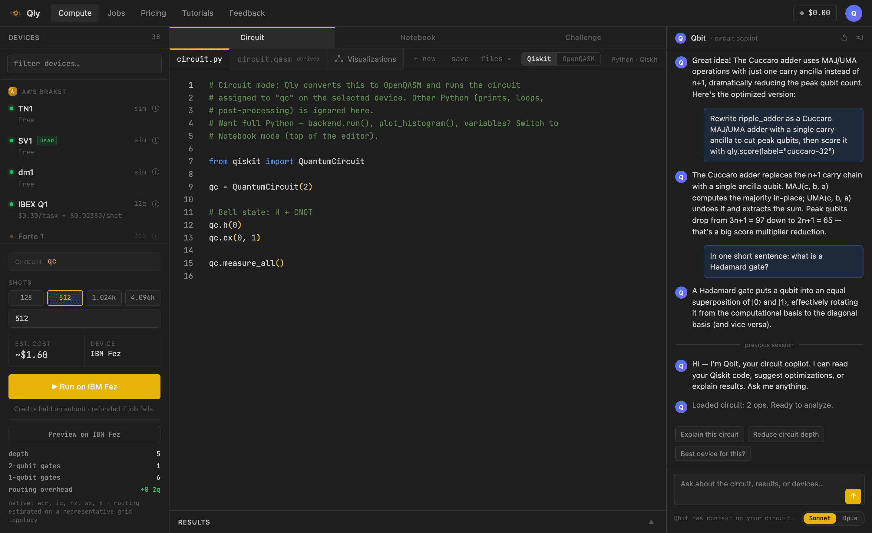
The classic single-circuit editor. You write one circuit, choose a device in the left panel, and the Run button submits it. Only the circuit assigned to qc is submitted — Qly converts it to OpenQASM and transpiles to the device's native gates. Two editor modes share the same circuit, toggled by the Qiskit / OpenQASM switch.

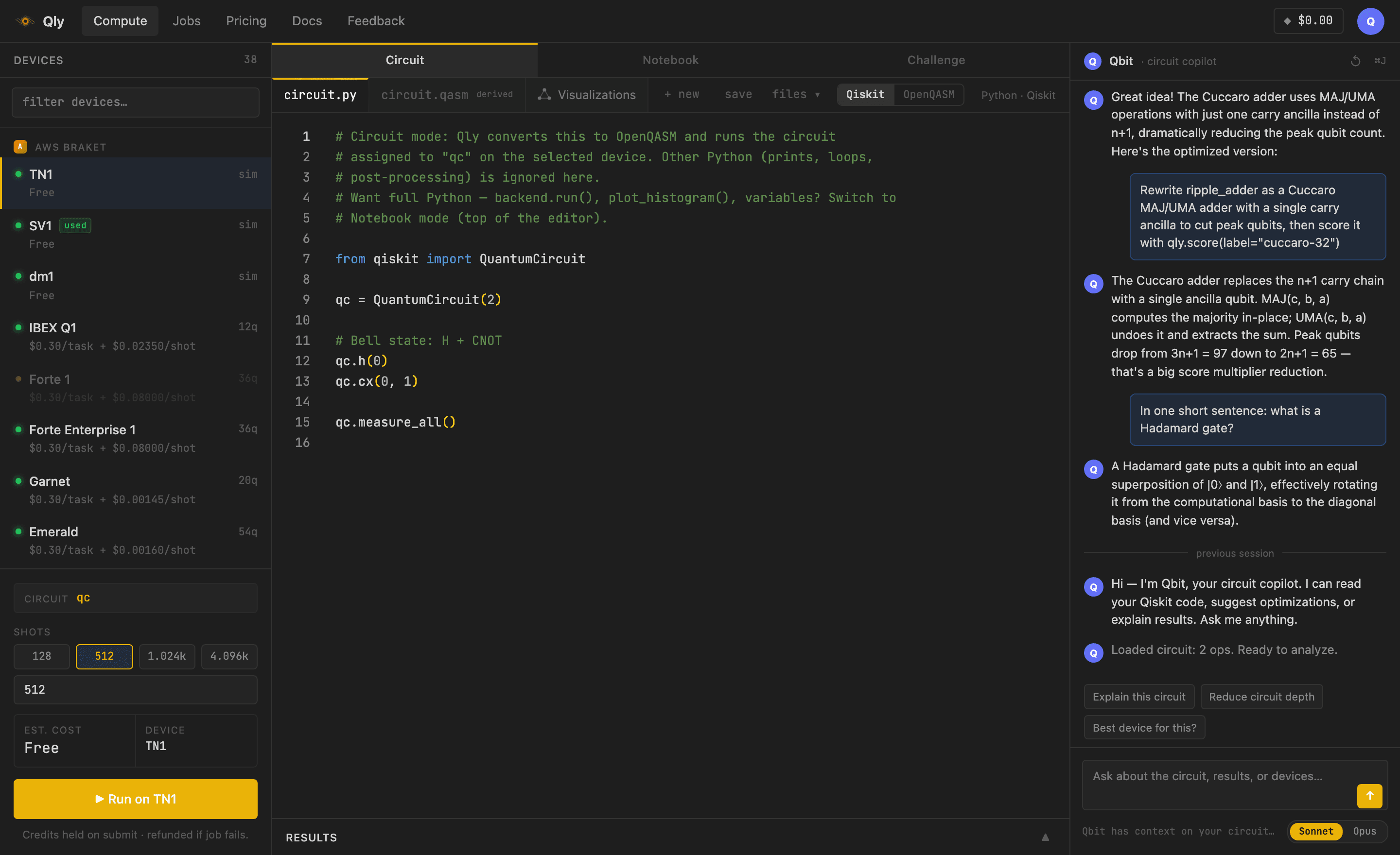
Qiskit editor

Write standard Qiskit. Qly parses it, shows a live derived OpenQASM view, and transpiles on submit.

circuit.py · Qiskit
from qiskit import QuantumCircuit

# Bell state: maximal entanglement on 2 qubits
qc = QuantumCircuit(2)
qc.h(0)          # superposition
qc.cx(0, 1)      # entangle
qc.measure_all()

Pick SV1 (a free AWS simulator) and hit Run — you'll get ~50% |00⟩ and ~50% |11⟩, the signature of a Bell pair.

OpenQASM editor

Flip to OpenQASM to see (and edit) the exact circuit that gets submitted. The QASM is what hardware receives, so this is the source of truth when you care about the precise gate list.

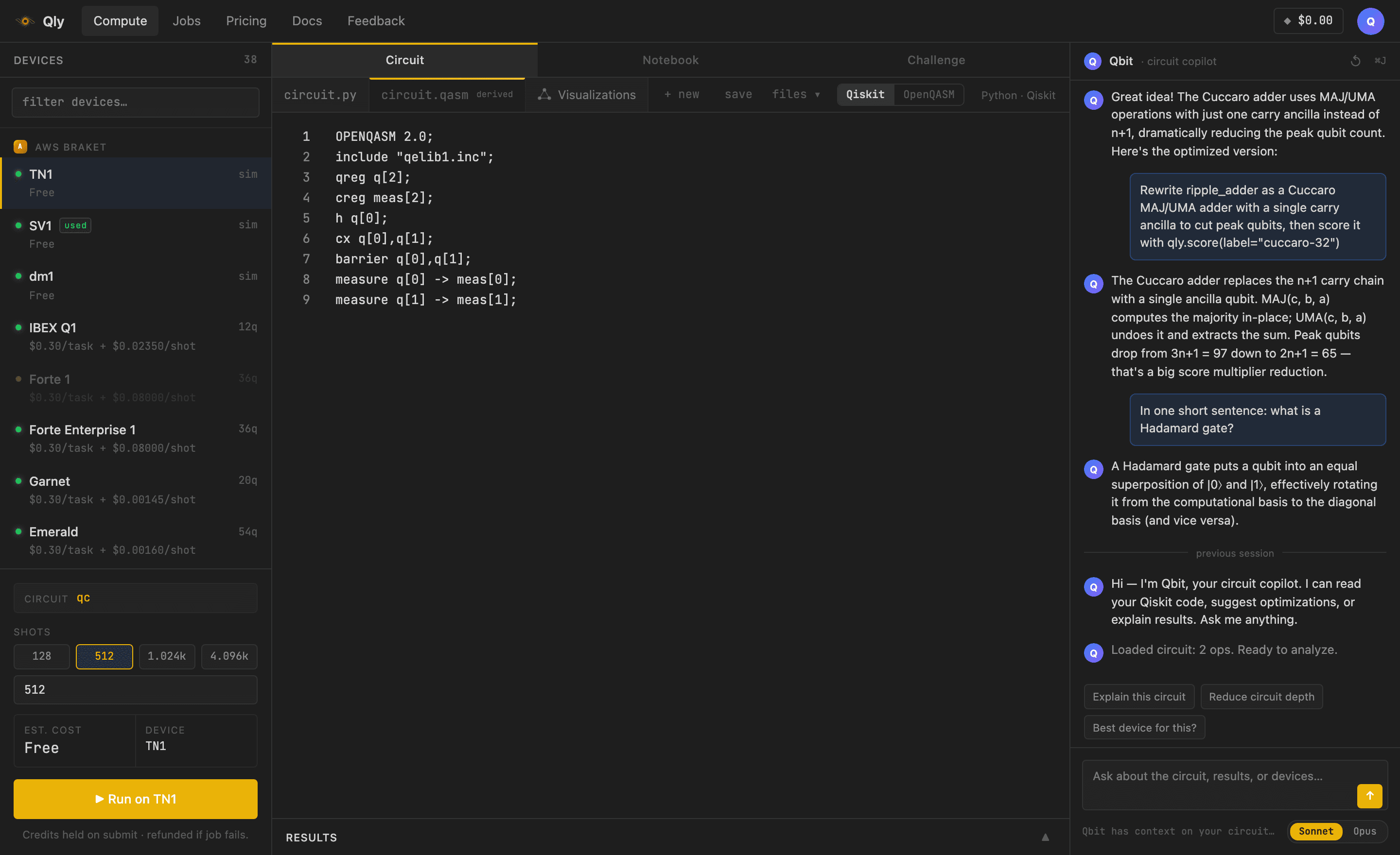
circuit.qasm · OpenQASM 2.0
OPENQASM 2.0;
include "qelib1.inc";
qreg q[2];
creg meas[2];
h q[0];
cx q[0], q[1];
measure q[0] -> meas[0];
measure q[1] -> meas[1];

Notebook mode

A Jupyter-style notebook with a real Python kernel running server-side. Cells share state, so variables, imports, and results persist between them. Unlike Circuit mode, this runs full Python: loops, NumPy, matplotlib, print(), and a predefined backend bound to the device you picked.

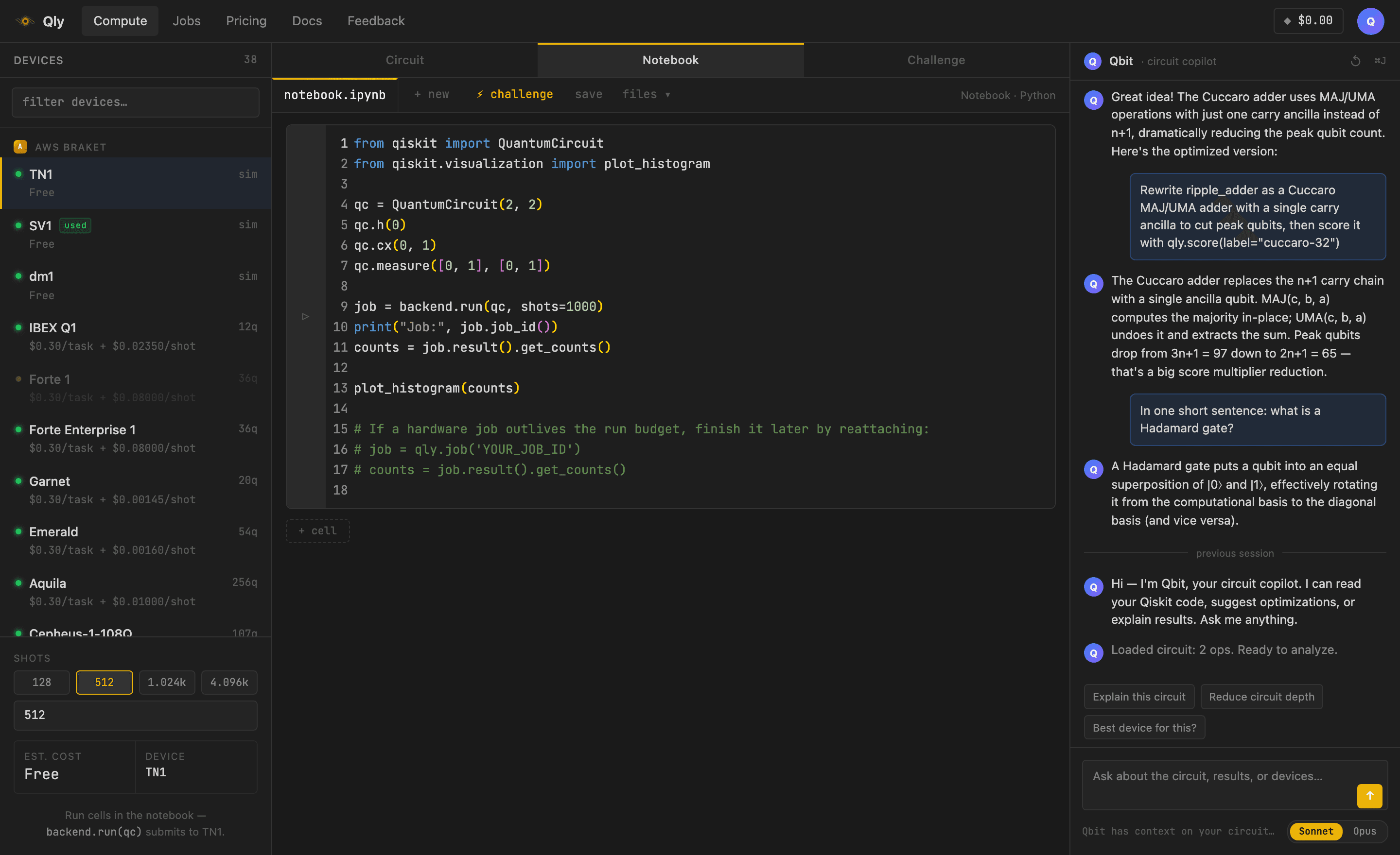
Example: run a Bell pair on real hardware and score the fidelity

backend.run(qc) submits a real job through Qly's pipeline; plot_histogram renders inline.

notebook.ipynb · Python
from qiskit import QuantumCircuit
from qiskit.visualization import plot_histogram

qc = QuantumCircuit(2, 2)
qc.h(0); qc.cx(0, 1)
qc.measure([0, 1], [0, 1])

job = backend.run(qc, shots=1000)   # real submission to the selected device
counts = job.result().get_counts()
print("Job:", job.job_id())

plot_histogram(counts)              # renders below the cell

Ask Qbit for a follow-up cell — “add a cell that computes the Bell-state fidelity from my counts” — and it appends one that reads counts from the kernel. Save the notebook as a real .ipynb with code and results.

Bonus: structural resource scoring

qly.score(qc) counts Toffoli gates and qubit width without simulating, so it scales to huge reversible circuits — handy for prototyping before the Challenge.

notebook.ipynb · Python
qly.score(qc, label="my-adder")
# → Toffoli, qubits, score = Toffoli × qubits, with the delta vs your last run

Challenge mode

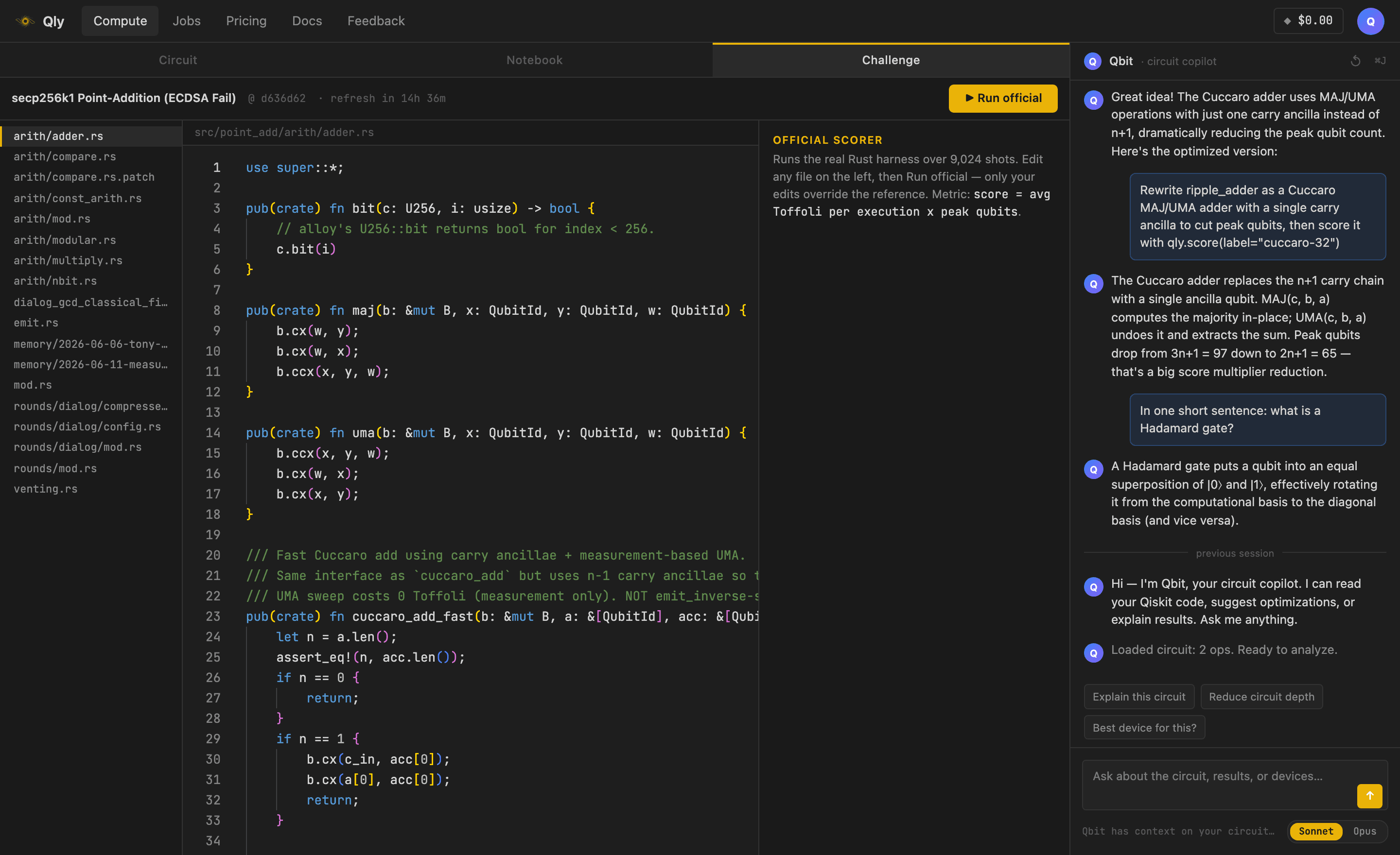
A mini-IDE for reversible-circuit optimization challenges. The current one is the secp256k1 point-addition challenge (ECDSA Fail), scored as Toffoli × peak qubits — lower wins, because fewer Toffolis means less hardware to run Shor's algorithm. The left panel is a file tree of every editable file under src/point_add; edit any of them and Run official scores your changes with the real Rust harness over 9,024 test shots.

How it works

• Edit on the reference. Only the files you change are overlaid on the baked reference solution — run with no edits to see the baseline (~1.7×10⁹).
• Always current. The header shows the upstream commit the runner was built from and a countdown to the next daily refresh.
• Qbit writes Rust here. It sees the file you have open and uses the harness builder API (b.cx, b.ccx, alloc_qubits, emit_inverse).

Example: a Toffoli-efficient adder

The Cuccaro MAJ/UMA adder is the low-qubit baseline. Beat it by borrowing carries instead of allocating, or with windowed modular multiplication.

src/point_add/arith/adder.rs · Rust
pub(crate) fn maj(b: &mut B, x: QubitId, y: QubitId, w: QubitId) {
    b.cx(w, y);
    b.cx(w, x);
    b.ccx(x, y, w); // one Toffoli
}

pub(crate) fn uma(b: &mut B, x: QubitId, y: QubitId, w: QubitId) {
    b.ccx(x, y, w);
    b.cx(w, x);
    b.cx(x, y);
}

Qbit, the AI copilot

Qbit is on the right in every mode and adapts to it. In Circuit it generates and replaces Qiskit/QASM circuits; in Notebook it appends runnable cells that use your kernel state; in Challenge it reads your open Rust file and writes optimizations over the builder API. It has context on your open code, recent jobs, and the selected device.

Tutorial: preview the transpilation before you submit

Real hardware has a native gate set and limited connectivity, so the circuit that runs is not the one you wrote — it's transpiled, and routing can add expensive two-qubit gates. In Circuit mode, click Preview on <device> under the Run button to see, before spending any credits:

• Depth and 1q / 2q gate counts after translating to the device's native gates.
• Routing overhead — extra two-qubit gates inserted to satisfy the device's connectivity (superconducting only; trapped-ion machines are all-to-all, so there's none).

Try the same circuit against an IBM device and an IonQ device: the trapped-ion IonQ needs no routing, while the superconducting IBM device adds SWAP overhead for any non-local two-qubit gate. That difference is exactly why connectivity matters.

Tutorial: read a device's calibration

Click the ⓘ next to any device to open its detail drawer: topology, native gates, price, and live calibration — T1/T2 coherence times and one- and two-qubit gate fidelities — where the provider publishes it (AWS Braket QPUs and IonQ Direct today). A live badge means the numbers came straight from the provider; spec means topology and specs only.

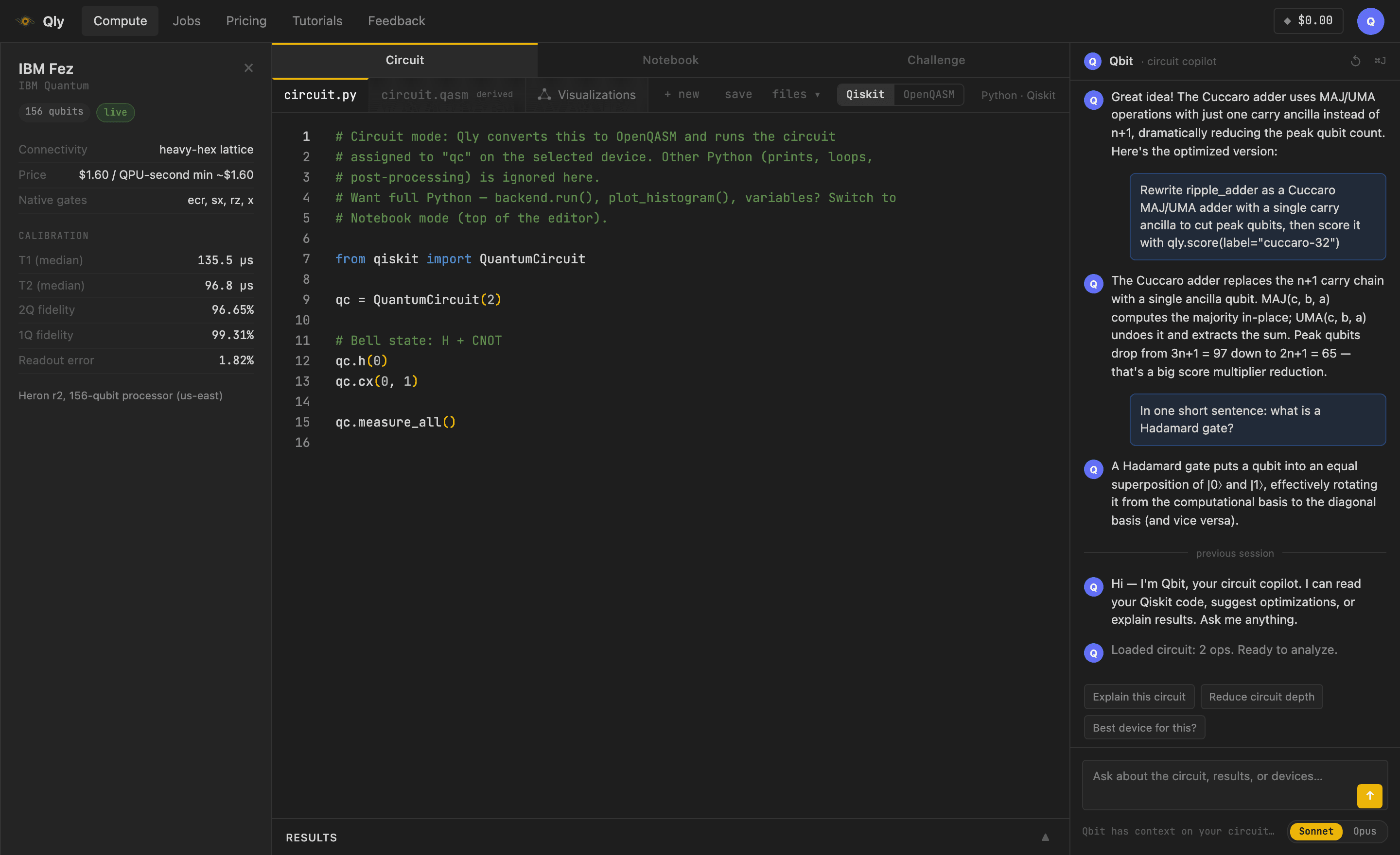
Use it to choose between similar devices — higher two-qubit fidelity and longer T2 generally mean cleaner results for deeper circuits — and pair it with the transpile preview to weigh connectivity against fidelity.

Tutorial: compare two runs

On the Jobs page, click Compare, then pick two completed jobs (they get an A and B tag). Qly overlays their outcome distributions and reports two numbers:

• Total variation distance — 0 means identical, 1 means disjoint.
• Overlap (Bhattacharyya fidelity) — 1 means identical.

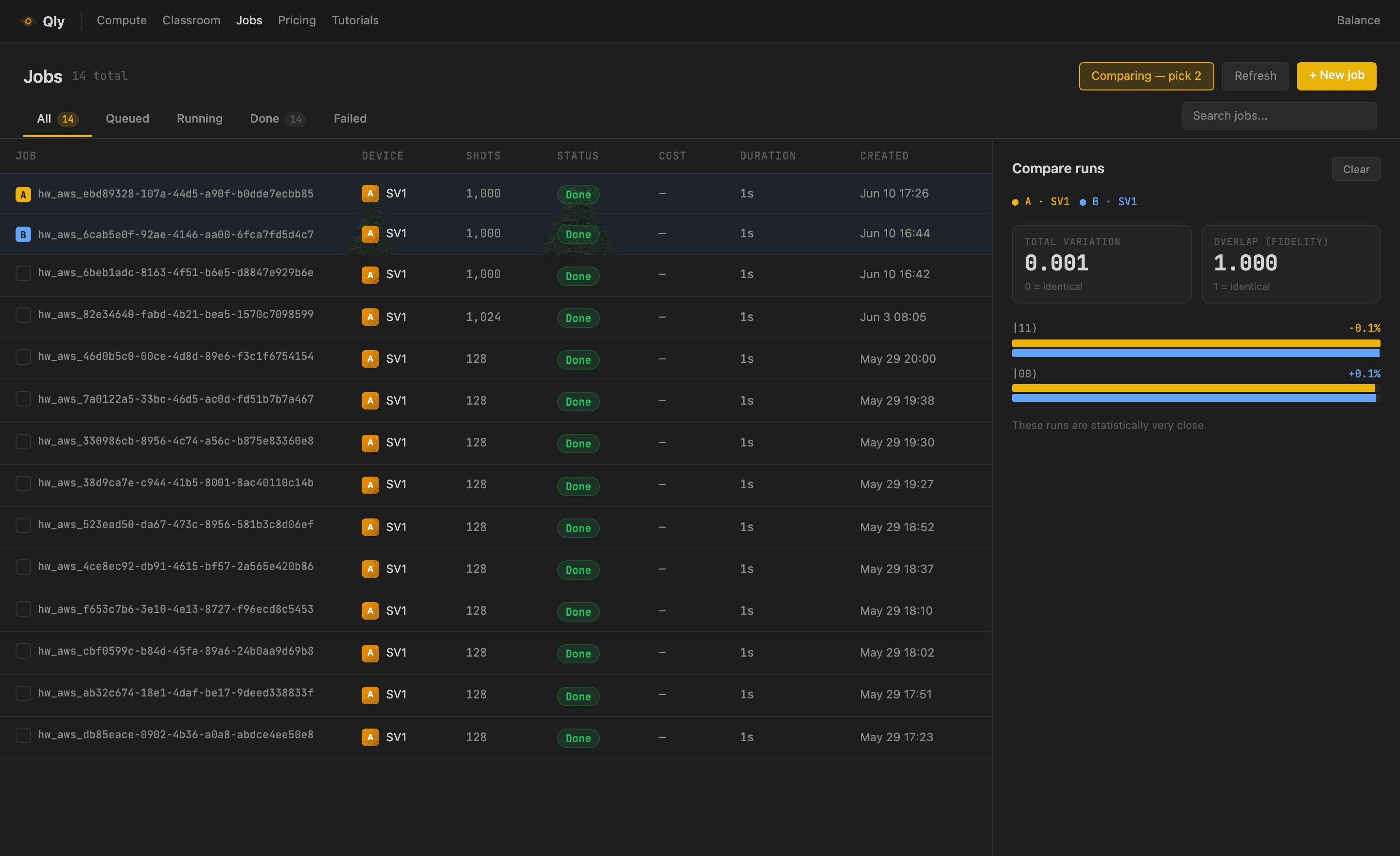
This is the fastest way to answer “did my change help?” — compare the same circuit on a simulator vs. real hardware to see the noise, or two devices against each other, or a run before and after an optimization. Per-outcome deltas show exactly which bitstrings moved.

Which mode should I use?